‘Navigation’ tab allows clickable navigation between all tabs in Excel file of the Model. By clicking on the block with any tab name, you will be instantly 'jumped' to that tab.

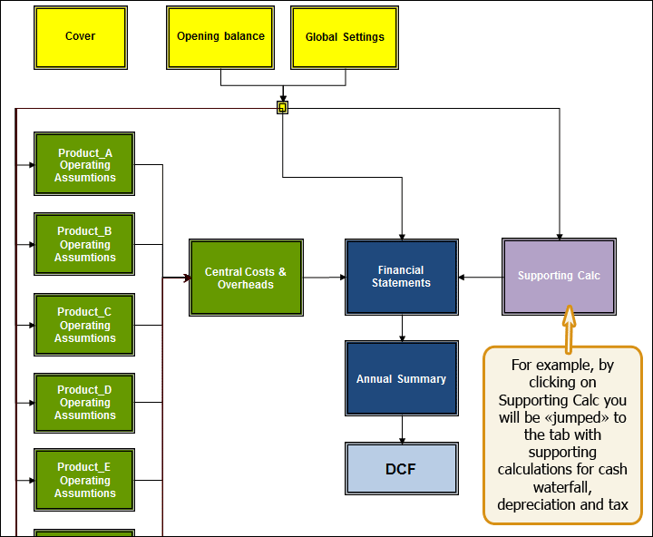
Figure 3.1. Navigation in the Excel file of the Model

Navigation hyperlink is located in the upper left corner of each tab. Clicking it will return you to 'Navigation' tab.

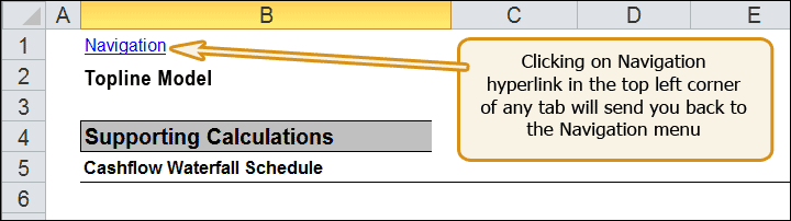
Figure 3.2. Upper left corner of ‘Supporting Calc' tab showing 'Navigation' link

To make hyperlinks work cell A1 in each tab has a hidden marker containing tab’s name. Although cell A1 appears empty, it is essential for the Model’s navigation to work properly. Do not remove this cell.

There are three fields at the centre of the tab. When the Model is opened for the first time, the fields show the following:

 Figure 3.3. Centre of 'Cover' tab showing default values

You can edit these legends by going to the tab called 'General Settings' ('Global'). At the top of ‘Global’ tab you can type in your own legends for the cover page, including the project name, version or date. The latter, unless manually overridden, will always show the current date whenever the file is re-opened.

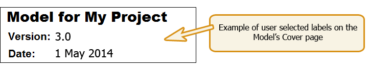
 Figure 3.4. Centre of 'Cover' tab showing new parameters

In addition to Cover settings described above, ‘Global’ tab contains general data inputs required by all other tabs of the Model to function properly.

If you populated all fields when assembling the Model online, there is nothing in the Global tab that requires your immediate attention. However, if you skipped some online Steps, ‘Global’ tab would be a good place to start populating the Model with your own data as follows:

Resetting the Model’s periodicity is for advanced users only. FinRobot does not guarantee the Model respond to change and will work correctly.

Figure 3.5. Inputs for the Model’s calendar and periodicity

Income tax, currency and units fields are located immediately below the calendar items.

All remaining editable areas of ‘Global’ tab - as described below - are labels for various line items used elsewhere in the Model. Unless changed during the assembly stage these will show default values. You can replace any default label with something more suitable for your business. Your inputs will be picked up throughout the Model automatically.

Figure 3.6. Relabeling COGS items

If you entered financial data for your opening balance sheet positions during the online assembly stage, then it will be present in the purchased Model and can be edited in this tab as required. Rates for working capital, cash and debt funding positions are also inputted in this tab alongside respective balance sheet line items.

If balance sheet structure for your business is more detailed or itemised than what is provided for in the Model, we advise you to aggregate similar line items.

If the total amounts of assets and liabilities match, then the check field at the bottom of the tab will be green and show 'OK'. If there is a mismatch, the check field will turn red and show the amount of discrepancy between the total assets and the total liabilities.

There is one more 'OK'/’Error’ check field at the top of 'Opening balance' sheet tab. ‘OK’ status indicates that balance sheets for all future dates in the financial statements of the Model are balanced. This integrated all-period check is reproduced in all tabs of the Model to alert users if a new input makes balance sheets 'to go off'.

The layout of Product / User tabs depends on your choice of how Revenues are modelled made at Step 1 during the online assembly stage. If at Step 1 you opted for sales channels then your Model will take the appearance shown in section 3.5.1 (Sales Channels). If your choice was customer dynamics’ option, then product tabs will look like those shown in section 3.5.2. (User Groups).

The number of tabs for product / user revenues and cost of goods sold (COGS) is determined by your choice made during the on-line assembly stage. The tabs are marked with letters from A to E. If only two product lines or user groups were ordered online then only ‘Product A’ and ‘Product B’ tabs will be present in the Model.

All product tabs or user group tabs are structurally equivalent. Online assembly populated all the tabs with identical data from your online entry for Product A or User Group A. You will need to review content of Product B to [E] and replace inputs with your own assumptions.

If during the online assembly stage you opted for sales channels option, your product tab would take the following appearance:

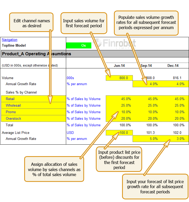
Figure 3.7. Top of Product tab – Sales Channel Option.

Note that the Model takes in growth rates expressed in annual terms. If your Model is quarterly or monthly, the Model will calendarise growth rates accordingly.

Separately, if you do not require revenues to be driven by both volume and pricing assumptions, you can set sales volume to 1 and assign 0% growth rate to the volume factor going forward. In such set up ‘List Price’ line will equal revenues (before discounts to channels).

Finally, you can assign various discounts and rebates to your sales channels as shown below. For example, retail or direct clients may have virtually no discounts to your list price while overstock gets sold at a very steep discount. If pricing strategy for your business differentiates by channel it obviously matters what sales volume allocation by channel is. You can change allocations over time to reflect different business objectives or seasonality patterns.

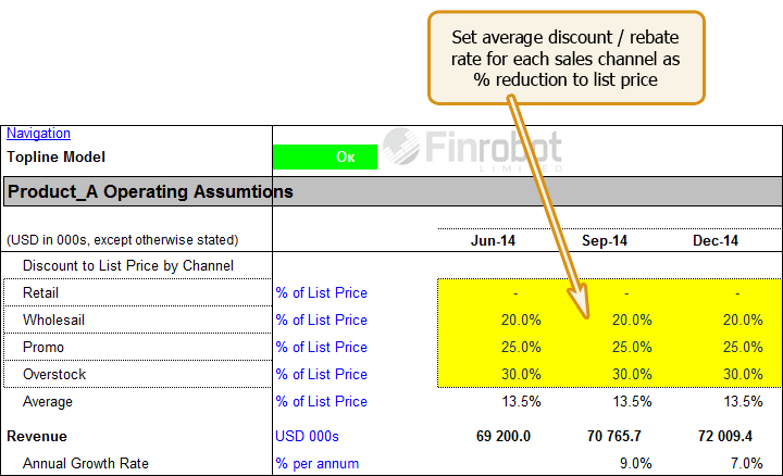
Figure 3.8. Applying price discounts to sales channels.

Your Revenue line is function of sales volume, pricing and discounts and channels mix going forward. If your change any of these assumptions Revenues will re-calculate accordingly.

This takes care of the top line. The product tab also contains inputs for Cost of Goods Sold as shown in the following picture.

Figure 3.9. Layout for COGS inputs.

Depending on choices made during online assembly you will see between one and five COGS line items preset to be either fixed or variable. Variable COGS are driven by cost per unit inflated at user determined rate whilst fixed COGS would run off an absolute base booked for the first forecast period.Note that when the downloaded Model is opened for the first time, growth and margin drivers are set flat over time but can be changed to any desired trajectory for each driver. For example, annual price growth may decelerate whilst costs as % of revenue may demonstrate improvements.

Note that when the downloaded Model is opened for the first time, growth and margin drivers are set flat over time but can be changed to any desired trajectory for each driver. For example, annual price growth may decelerate whilst costs as % of revenue may demonstrate improvements. 

If during online assembly you opted for customer dynamics option, your product tab would take the following appearance:

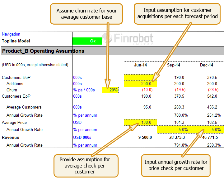
Figure 3.10. Top of Product tab – Customer Dynamics Option.

Your top line runs off customer dynamics assumptions. Every period some customers are acquired and some customers churn away from your customer base for good. Applying average check per customer to average customers for each period yields revenue figure as shown at the bottom of the above diagram.

Note that unlike volume / pricing module assumed for Sales Channels your Customer driven Revenue line is non-linear as it is a function how fast customers can be acquired to compensate for churn of your customer base. You can smooth the trajectory by calibrate acquisition assumption and the churn rate but it is unlikely to produce a straight a straight line.

This takes care of the top line. The user group version of the product tab also contains inputs for Cost of Goods Sold. The layout is identical to the one shown in Figure 3.9 above. Note that if you choose to drive your COGS items as variable drivers (per user), the total for each COGS item may show material swings as your customer base gyrates over time.

'Central Costs' tab contains inputs and calculations related overhead and central costs items such as administrative and marketing expenses.

The structure and computations should match the assumptions provided during the on-line assembly stage – please refer to Section 2 of the Manual for details. If you skipped input entries during online assembly, then your Model would contain dummy numbers. Depending on your selection online each cost element is forecast forward as either variable or fixed as shown in the diagram below:

Figure 3.11. Central Costs and Overhead assumptions

Note that when the downloaded Model is opened for the first time, growth and margin drivers are set flat over time. You can assume any desired trajectory for each driver. For example, annual revenue growth may decelerate whilst costs as % of revenue may demonstrate improvements.

Note that the Model takes in growth rates expressed in annual terms. If your Model is quarterly or monthly, the Model will calendarise growth rates accordingly.

‘Supporting Calc’ tab keeps all supporting financial calculations in one place. These are cash waterfall, tax / loss carry-forwards, working capital requirements and CapEx/Depreciation schedules.

If you start from the top of the tab, the first schedule will look like the following:

Figure 3.12. Cash Waterfall

You can use this schedule to assume minimum amount of cash required in the business at any time. The Model will take care of the rest as the next schedule will automatically works out debt borrowings and repayments based on cash available / required shown at the bottom of the waterfall.

If you wish to change assumptions for cash and debt rates, you can do so by goring to 'Opening Balance' sheet tab. Note that rates are expressed in annual terms and automatically calendarise depending on the chosen periodicity of the Model. There is no need to adjust anything if your Model is quarterly or monthly.

By default, any period interest charge for any debt obligation is calculated based on the opening position. If there are large fluctuations due to borrowing and/or repayments with a period this method may not be a good proxy for what is actually expected. However, the Model can calculate more accurate interest charges based on average debt positions. This would require the Model to go circular by turning on the cyclical interest calculation switch. The switch is located in the upper left corner of 'Financials' tab. Note, that if the switch is on, then Excel settings (options) should have iterations (cyclical) options turned on too.

The next area of the Supporting Calc tab is a tax calculater containing workings for your tax liability and cash tax payments for each forecast period. The schedule takes earnings before tax from 'Financials' tab, allows for manual adjustment to reported earnings, and finally provides for any loss carried forward in case there is a taxable loss in any given period, which can be carried forward and offset against taxable income in the future.

The default assumption is that taxable turnover matches the reported in 'Financial' tab, and no manual adjustments are necessary.

FinRobot does not provide tax advice and the Model is not attempting to represent a real tax environment. You should seek advice from a tax specialist if you wish to model a tax environment compliant with tax laws and regulations relevant to your business.

The last table in the tab contains all inputs and workings necessary to drive investment and depreciation, which are fed into financials. Provide assumptions for your future CapEx programme (as negative), set deprecation rates for existing and new investments, and the Model will take care of the rest.

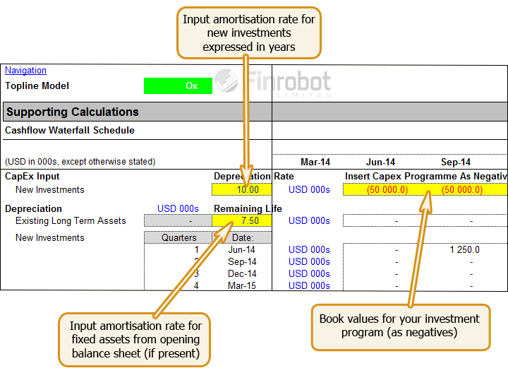
Figure 3.13 CapEx and Depreciation Assumptions

'Financials' tab contains three standard financial reports, viz. profit and loss, balance sheet and cash flows. The tab does not require user inputs except for Exceptional Items and Equity distributions as described below. All other data are picked up from tabs covered in the preceding sections of the Manual.

The financial statements are purposefully generic. As our clients are located in various countries and operate under different accounting standards we cannot make the Model comply to a specific accounting standard.

Instead, we make reports relatively simple and easy to navigate or to adjust if needed. Our experience shows that the majority of our clients are satisfied with our approach, particularly for the purposes of preparing management accounts and/or investment decision analysis.

The Net Exceptional Item allows for manual entry of exceptional items, which are not practical to model, but are known occurrences within the forecast period. For example, a known gain from disposing of non-core other assets. Note that the Model implicitly assumes that any exceptional loss or gain is a cash item. If your circumstances are such that an exceptional item is a non-cash expense, you need (i) to disconnect the link between extraordinary P&L items and extraordinary cash flow items and (ii) to link your extraordinary P&L item to a corresponding line of the balance sheet (e.g. write off a balance sheet position). Note that such adjustments would require good working knowledge of the Model. Otherwise, there is a risk that the balance sheet would 'go off' and the check flag would indicate red.

The Equity Issue line of the cash flow allows for manual entry of any forecast cash distributions (dividends or buybacks) or capital fundraising (issue). A positive entry means equity is raised. Negative means cash is returned to shareholders. If you wish to use the line for a dividend programme, it is possible to link up the cash flow equity line to a % net income from P&L.

Finally, ‘Financials’ tab has an iterative calculations switch. Please refer to section 3.8 above for details.

Annual Summary' tab is designed to automatically aggregate data for monthly and quarterly models into an annual summary. The tab does not require any user input.

Please note that if your monthly or quarterly forecast periods do not accrue to full number of years, the last forecast year in 'Annual Summary' tab will pick up the residual period of less than one full year.

The minimum number of years shown in 'Annual Summary' tab is three. Hence, if your project is less than two years you are likely to see 0 in the last column of the summary. Note that for any length of the project the summary would pick up last available projected balance sheet irrespective whether its date falls on a year end, or not.

'DCF Analysis' tab provides valuation metrics with respect to your project or business as outlined in the Model. The outputs are presented in grid form for Firm Value and Equity Value based on DCF approach. IRR analysis is presented on Firm Value basis only.

Additional analysis is available with respect to the terminal value for going concern exit value. You can compare implied perpetuity growth to assumed multiple for terminal value and vice verse.

'DCF Analysis' tab picks up the data from 'Annual Summary' tab. Hence, all financial information is presented on annual basis irrespective of the underlying periodicity of the Model.

Please note that if your project is finite and its length does not accrue to full years of forecast, then NPV and IRR may require adjustments as set out below. For projects with duration of less than two years, we advise setting Terminal Value to zero. 

To run and interpret data with the help of 'DCF Analysis' tab please consider the following:

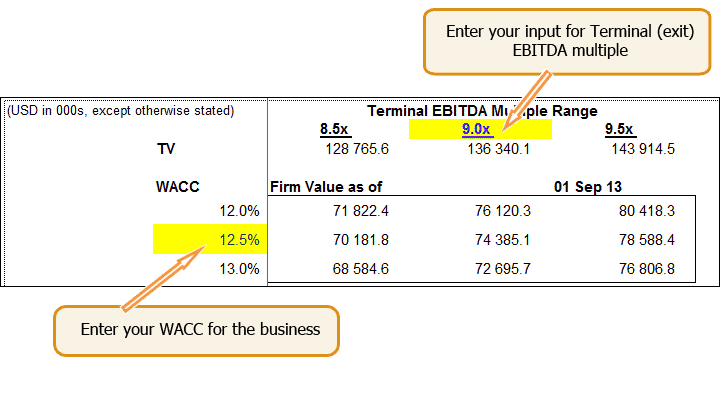
          Figure 3.14. WACC and exit multiple assumptions

IRR function implies that either there is some invested capital upfront or that first period cash flow is a negative. If this is not the case, for example, you project shows positive cash flows for all periods and requires no upfront capital IRR calculation would return an error.